Time series plot

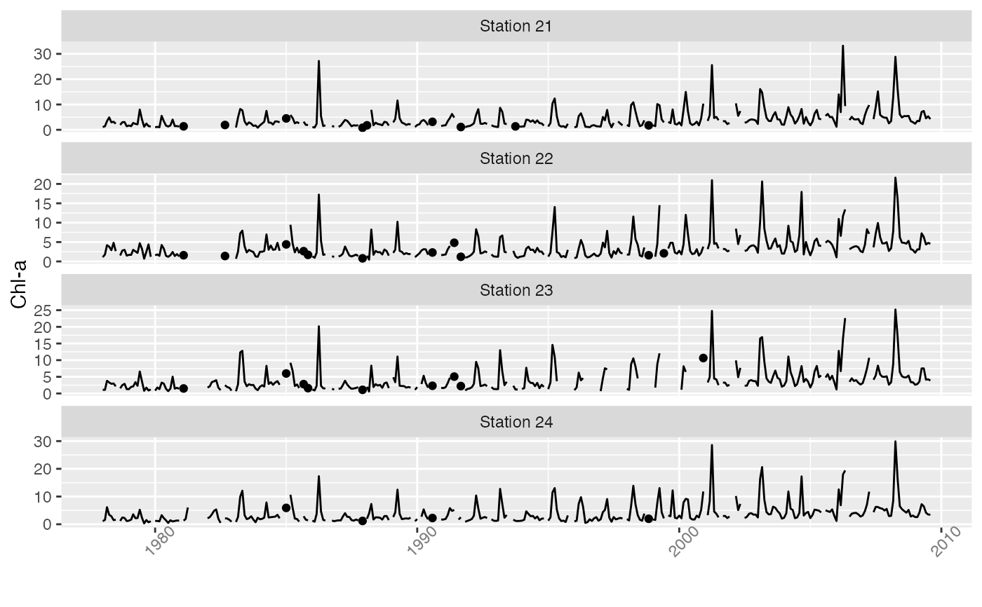
Creates line plot of vector or matrix time series, including any data surrounded by NAs as additional points.

plotTs(
  x,
  dot.size = 1,
  xlab = NULL,
  ylab = NULL,
  strip.labels = colnames(x),
  ...
)

Arguments

x

matrix or vector time series

dot.size

size of dots representing isolated data points

xlab

optional x-axis label

ylab

optional y-axis label

strip.labels

labels for individual time series plots

...

additional options

Value

A plot or plots and corresponding object of class “ggplot”.

Details

The basic time series line plot ignores data points that are adjacent to missing data, i.e., not directly connected to other observations. This can lead to an uninformative plot when there are many missing data. If one includes both a point and line plot, the resulting graph can be cluttered and difficult to decipher. plotTs plots only isolated points as well as lines joining adjacent observations.

Options are passed to the underlying facet_wrap function in ggplot2. The main ones of interest are ncol for setting the number of plotting columns and scales = "free_y" for allowing the y scales of the different plots to be independent.

See also

plotTsAnom

Author

Alan Jassby, James Cloern

Examples

# Chlorophyll at 4 stations in SF Bay
chl <- sfbayChla[, 1:4]
plotTs(chl, dot.size = 1.5, ylab = 'Chl-a', strip.labels = paste('Station',
  substring(colnames(chl), 2, 3)), ncol = 1, scales = "free_y")