rv: a simulation-based random variable class
Jouni Kerman
2022-02-13
Source:vignettes/rv-doc.Rmd
rv-doc.RmdEdited by Jemma Stachelek: 13 February, 2022
rv is an implementation of a simulation-based random variable object class for R, originally introduced in Kerman and Gelman (2007).
rv implements a new class of vectors that contain a ‘hidden dimension’ of simulations in each scalar component. These rv objects can be manipulated much like any numeric vectors, but the arithmetic operations are performed on the simulations, and summaries are calculated from the simulation vectors.
rv is convenient for manipulating posterior simulations obtained from MCMC samplers, for example using Umacs (Kerman 2005) or R2WinBUGS (Sturtz, Ligges, and Gelman 2005) (the package provides a coercion method to convert bugs objects to rv objects.)
The paper by Kerman and Gelman (2007) introduces the principles of the design of random variable objects. This document is a short overview of some of the commands provided by the package rv. At the end of the document there is a short description of the implementation.
Installation
Install the package rv (version 2.1.1 or higher) using the Package Installer command in R (from the menu), and load the package using,
A quick tour
The rv objects (or, “random vectors”) that we manipulate usually come from a Markov chain sampler. To introduce some commands quickly, we will instead use some random vectors generated by random-vector generating functions which sample directly from a given (standard) distribution.
Number of simulations.
First, we will set the number of simulations we use. We choose 4000 simulations per each scalar component of a random vector:
setnsims(4000)
#> [1] 4000
We will not usually change this value during our session, unless we want to repeat our analysis with more (or fewer) simulations. The default value is 4000, set whenever the package is loaded for the first time in the workspace; therefore this is not strictly a necessary step to do every time we start the package.
A Normally distributed random vector
To draw a random Gaussian (Normal) vector of length 5 with corresponding means \(1,2,3,4,5\) and s.d. 1,
x <- rvnorm(mean=1:5, sd=1)In effect, the object x now contains five vectors of length \(4000\), drawn (internally) using rnorm, but we see x as a vector of length 5.
The length of the vector is derived from the length of the mean vector (and the sd vector), and it is not necessary to specify a parameter “n”.
Quick distribution summary
To summarize the distribution of x by viewing quantiles, means, and s.d.’s, we only type the name of the object at the console:
x
#>     mean   sd    1%   2.5%  25% 50% 75% 97.5% 99% sims
#> [1] 0.98 0.98 -1.35 -0.926 0.31   1 1.7   2.9 3.2 4000
#> [2] 1.98 1.01 -0.40  0.015 1.28   2 2.7   3.9 4.3 4000
#> [3] 3.02 0.99  0.76  1.059 2.35   3 3.7   5.0 5.2 4000
#> [4] 4.02 1.01  1.64  1.983 3.35   4 4.7   5.9 6.3 4000
#> [5] 4.99 0.97  2.77  3.144 4.33   5 5.7   6.9 7.2 4000
Similarly we can draw from Poisson (rvpois) Gamma, (rvgamma), Binomial (rvbinom):
y <- rvpois(lambda=10)Componentwise summaries
To extract the means, we use rvmean, the s.d.’s, we use rvsd, the minimum, rvmin, the maximum rvmax, and the quantiles, we use rvquantile. The componentwise medians are also obtained by rvmedian:
rvmean(x)
#> [1] 0.98 1.98 3.02 4.02 4.99
rvsd(x)
#> [1] 0.98 1.01 0.99 1.01 0.97
rvquantile(x, c(0.025,0.25,0.5,0.75,0.975))
#>        2.5%  25% 50% 75% 97.5%
#> [1,] -0.926 0.31   1 1.7   2.9
#> [2,]  0.015 1.28   2 2.7   3.9
#> [3,]  1.059 2.35   3 3.7   5.0
#> [4,]  1.983 3.35   4 4.7   5.9
#> [5,]  3.144 4.33   5 5.7   6.9
rvmedian(x)
#> [1] 1 2 3 4 5
rvmin(y)
#> [1] 1
rvmax(y)
#> [1] 24
For convenience, there is an alias E(...) for rvmean(...) which gives the “expectation” of a random vector.
Note
Since the random vectors are all represented by simulations, the expectation and all other functions that we compute are just numerical approximations. Generating a “standard normal random variable” with z <- rvnorm(n=1, mean=0, sd=1) will not have an expectation exactly zero. Our main purpose here is to handle simulations, so the answers will be approximate and necessarily involve a simulation error.
Extracting and replacing
Since rv objects work just like vectors, we can extract and replace components by using the bracket notation. Here we replace the 3rd and 4th components with random variables having (an approximate) binomial distributions:
x[3:4] <- rvbinom(size = 1, prob = c(0.1, 0.9))
x[3:4]
#>     mean   sd 1% 2.5% 25% 50% 75% 97.5% 99% sims
#> [1]  0.1 0.30  0    0   0   0   0     1   1 4000
#> [2]  0.9 0.31  0    0   1   1   1     1   1 4000
The “mean” column now shows the estimate of the expectation of the two indicator functions we generated.
Imputing into regular vectors
To “impute” a random vector in a regular numeric vector, we can either first turn the constant vector into an rv object:
y <- as.rv(1:5)
y[3:4] <- x[3:4]
y
#>     mean   sd 1% 2.5% 25% 50% 75% 97.5% 99% sims
#> [1]  1.0 0.00  1    1   1   1   1     1   1    1
#> [2]  2.0 0.00  2    2   2   2   2     2   2    1
#> [3]  0.1 0.30  0    0   0   0   0     1   1 4000
#> [4]  0.9 0.31  0    0   1   1   1     1   1 4000
#> [5]  5.0 0.00  5    5   5   5   5     5   5    1
or, use the special function impute that can handle regular vectors and rv objects:
y <- (1:5)
impute(y, 3:4) <- x[3:4]
y
#>     mean   sd 1% 2.5% 25% 50% 75% 97.5% 99% sims
#> [1]  1.0 0.00  1    1   1   1   1     1   1    1
#> [2]  2.0 0.00  2    2   2   2   2     2   2    1
#> [3]  0.1 0.30  0    0   0   0   0     1   1 4000
#> [4]  0.9 0.31  0    0   1   1   1     1   1 4000
#> [5]  5.0 0.00  5    5   5   5   5     5   5    1
The non-random components appearing as “constants,” or in other words, random variables with point-mass distributions (and therefore having a zero variance).
Summaries of functions of random vectors
Standard numerical functions can be applied directly to random vectors. To find a summary of the distribution of the function \(1/(1+\exp(-x_1))\), we would write,
1/(1 + exp(-x[1]))
#>     mean   sd   1% 2.5%  25%  50%  75% 97.5%  99% sims
#> [1] 0.69 0.18 0.21 0.28 0.58 0.73 0.84  0.95 0.96 4000
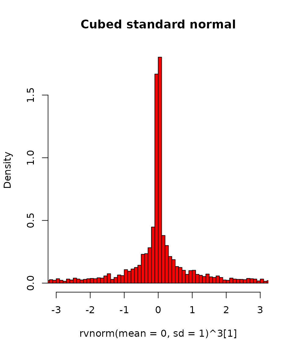
Or of the function of almost anything we like:
Order statistics
To simulate the order statistics of a random vector x, we can use sort(x), min(x), max(x).
x <- rvpois(lambda=1:5)
x
#>     mean  sd 1% 2.5% 25% 50% 75% 97.5% 99% sims
#> [1] 0.98 1.0  0    0   0   1   2     3   4 4000
#> [2] 1.98 1.4  0    0   1   2   3     5   6 4000
#> [3] 2.97 1.7  0    0   2   3   4     7   8 4000
#> [4] 3.96 2.0  0    1   3   4   5     8   9 4000
#> [5] 5.03 2.2  1    1   3   5   6    10  11 4000
sort(x)
#>     mean   sd 1% 2.5% 25% 50% 75% 97.5% 99% sims
#> [1] 0.61 0.69  0    0   0   0   1     2   2 4000
#> [2] 1.62 0.91  0    0   1   2   2     3   4 4000
#> [3] 2.72 1.07  1    1   2   3   3     5   5 4000
#> [4] 4.02 1.29  2    2   3   4   5     7   7 4000
#> [5] 5.96 1.83  3    3   5   6   7    10  11 4000
min(x)
#>     mean   sd 1% 2.5% 25% 50% 75% 97.5% 99% sims
#> [1] 0.61 0.69  0    0   0   0   1     2   2 4000
max(x)
#>     mean  sd 1% 2.5% 25% 50% 75% 97.5% 99% sims
#> [1]    6 1.8  3    3   5   6   7    10  11 4000
Note: the order method is not implemented.
Random matrices and arrays
rv objects behave like numerical vectors in R; thus you can set their dimension attributes to make them appear as arrays, and also use the matrix multiplication operator. (Note: \%**\%} performs the matrix multiplication, ensuring that non-rv andrvobjects get properly multiplied. Using%*%` does not work if the
matrix or vector on the left is not an rv object.)
p <- runif(4) # Some prior probabilities.
y <- rvbinom(size=1, prob=p) # y is now a rv of length 4.
dim(y) <- c(2,2) # Make y into a 2x2 matrix.
y
#>         mean   sd 1% 2.5% 25% 50% 75% 97.5% 99% sims
#> [1,1] 0.3435 0.47  0    0   0   0   1     1   1 4000
#> [2,1] 0.1010 0.30  0    0   0   0   0     1   1 4000
#> [1,2] 0.4225 0.49  0    0   0   0   1     1   1 4000
#> [2,2] 0.0065 0.08  0    0   0   0   0     0   0 4000
y %**% y
#>        mean   sd 1% 2.5% 25% 50% 75% 97.5% 99% sims
#> [1,1] 0.385 0.51  0    0   0   0   1     1   2 4000
#> [2,1] 0.032 0.18  0    0   0   0   0     1   1 4000
#> [1,2] 0.147 0.36  0    0   0   0   0     1   1 4000
#> [2,2] 0.048 0.21  0    0   0   0   0     1   1 4000
The componentwise summary functions such as E (rvmean) and rvsd return the summaries with the correct dimension attribute set:
E(y)
#>      [,1]   [,2]
#> [1,] 0.34 0.4225
#> [2,] 0.10 0.0065
Creating indicator functions with logical operations
Applying logical operators gives indicators of events. If z is a standard normal random variable the indicator of the event \(\{z>1\}\) is given by the statement z>1:
z <- rvnorm(1)
z > 1
#>     mean   sd 1% 2.5% 25% 50% 75% 97.5% 99% sims
#> [1] 0.14 0.35  0    0   0   0   0     1   1 4000
We can also use the convenience function Pr(...) to compute the estimates of the expectation of these indicators:
Pr(z > 1)
#> [1] 0.14
Of course, we can find joint events as well and computer their probabilities similarly. To find the probability that \(Z_1>Z_2^2\), where both \(Z_1\) and \(Z_2\) are independent standard normal, we’d type
We can even compute probabilities of intersections or unions of events,
Functions of several random variables
We can use random vectors, regular vectors, standard elementary functions, logical operations in any combination as we wish.
Example. Let \(z_1,z_2\) be standard normal, and let \(y_1=\exp(z_1), y_2=y_1\exp(z_2)\).
Compute the expectation of \(x=(y_1-1)\mathrm{1}_{y_1>1}\mathrm{1}_{y_2>1}\) and find the probability \(\Pr(x>1)\).
Posterior simulations from a classical regression model
We can generate posterior simulations from a classical regression model, using the standard assumptions for the priors. For convenience there is a function posterior to do this.
  n <- 10
  ## Some covariates
  X <- data.frame(x1=rnorm(n, mean=0), x2=rpois(n, 10) - 10)
  y.mean <- (1.0 + 2.0 * X$x1 + 3.0 * X$x2)
  y <- rnorm(n, y.mean, sd=1.5) ## n random numbers
  D <- cbind(data.frame(y=y), X)
  ## Regression model fit
  fit <- lm(y ~ x1 + x2, data=D)
The Bayesian estimates (posterior distributions) are represented by,
  Post <- posterior(fit)
  Post
#> $beta
#>            name mean   sd    1%  2.5%  25% 50% 75% 97.5% 99% sims
#> [1] (Intercept)  1.1 0.80 -0.91 -0.45 0.56 1.0 1.5   2.7 3.1 4000
#> [2]          x1  2.0 0.71  0.19  0.57 1.58 2.0 2.4   3.4 3.8 4000
#> [3]          x2  2.9 0.22  2.33  2.43 2.77 2.9 3.0   3.3 3.4 4000
#>
#> $sigma
#>     mean   sd   1% 2.5% 25% 50% 75% 97.5% 99% sims
#> [1]  1.7 0.54 0.91 0.97 1.3 1.6 1.9     3 3.5 4000
Creating replicated simulations
Continuing the previous example, we’ll resample from the sampling distribution of \(y\) using the posterior simulations we got. We can use the function rvnorm to do this, since it accepts random vectors as arguments. Rather than think rvnorm to draw normal random vectors, it rather “samples from the normal model.” The vector will be normal given (constant) mean and s.d., but if the mean and s.d. are not constants, the resulting vector will not be normal.
sigma <- Post$sigma
betas <- Post$beta
M <- model.matrix(fit)
y.rep <- rvnorm(mean=M %**% betas, sd=sigma)
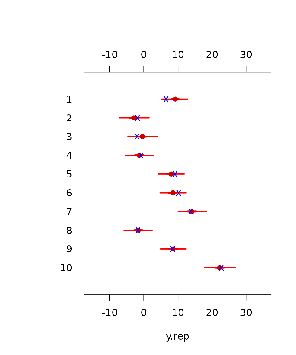
mlplot(y.rep) # Summarize graphically.
Note also that
 sigma is also an rv object.
The matrix multiplication statement returns a random vector of length :
M %**% betas
#>      name  mean   sd   1% 2.5%  25%  50%   75% 97.5%   99% sims
#>  [1]    1  9.14 0.74  7.2  7.6  8.7  9.1  9.58 10.65 11.07 4000
#>  [2]    2 -2.95 1.24 -6.1 -5.4 -3.7 -3.0 -2.20 -0.41  0.18 4000
#>  [3]    3 -0.41 1.19 -3.3 -2.7 -1.1 -0.4  0.27  2.05  2.61 4000
#>  [4]    4 -1.34 1.00 -3.7 -3.3 -1.9 -1.3 -0.76  0.76  1.20 4000
#>  [5]    5  7.99 0.56  6.6  6.9  7.6  8.0  8.33  9.14  9.41 4000
#>  [6]    6  8.49 0.62  6.9  7.3  8.1  8.5  8.86  9.76 10.12 4000
#>  [7]    7 14.06 1.01 11.4 12.0 13.5 14.1 14.67 16.10 16.58 4000
#>  [8]    8 -1.63 0.91 -3.8 -3.4 -2.2 -1.6 -1.08  0.24  0.76 4000
#>  [9]    9  8.53 0.63  7.0  7.3  8.2  8.5  8.91  9.82 10.18 4000
#> [10]   10 22.25 1.33 18.7 19.4 21.5 22.3 23.05 24.90 25.40 4000
Thus all the uncertainty in the mean estimate \(X\beta\) and the residual s.d. estimate \(\sigma\) is propagated when the replicated vector \(y^\mathrm{rep}\) is generated. In effect, this single line of code thus will in fact draw from the distribution \(p({y}^\mathrm{rep}|y)=\int\int \mathrm{Normal}({y}^\mathrm{rep}|\mu,\sigma)p(\mu,\sigma|y)\mathrm{d}\mu\mathrm{d}\sigma.\)
For convenience, there is a generic method rvpredict to generate replications and predictions:
  ## Replications
  y.rep <- rvpredict(fit)
We can also generate predictions at some other covariate values:
  ## Predictions at the mean of the covariates
  X.pred <- data.frame(x1=mean(X$x1), x2=mean(X$x2))
  y.pred <- rvpredict(fit, newdata=X.pred)
We can also perturb (add uncertainty to) the covariate `x1}, then predict again.
  X.rep <- X
  X.rep$x1 <- rnorm(n=n, mean=X.rep$x1, sd=sd(X.rep$x1))
  y.pred2 <- rvpredict(fit, newdata=X.rep)
  y.pred2
#>        mean  sd    1% 2.5%    25%    50%  75% 97.5%  99% sims
#>  [1] 13.143 2.1   8.1  8.9 11.833 13.134 14.4 17.56 18.7 4000
#>  [2] -2.326 2.0  -7.5 -6.3 -3.556 -2.333 -1.1  1.65  2.6 4000
#>  [3]  1.479 2.4  -4.5 -3.4  0.024  1.508  3.0  6.05  7.1 4000
#>  [4]  0.053 2.1  -5.3 -4.4 -1.213  0.037  1.4  4.34  5.3 4000
#>  [5]  9.236 2.0   4.3  5.3  8.095  9.214 10.4 13.13 14.3 4000
#>  [6]  7.907 1.8   3.4  4.2  6.778  7.895  9.0 11.70 12.5 4000
#>  [7] 12.812 2.2   7.3  8.4 11.506 12.850 14.1 16.95 18.0 4000
#>  [8] -4.792 2.6 -11.1 -9.8 -6.347 -4.801 -3.3  0.39  1.9 4000
#>  [9]  7.426 1.9   2.4  3.6  6.296  7.472  8.6 10.93 12.0 4000
#> [10] 20.114 2.2  14.5 15.8 18.832 20.110 21.4 24.62 25.9 4000
Graphical summaries}
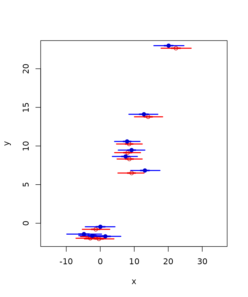
Graphical summaries are still in development, but it is now possible to plot a scatterplot with a regular vector against a random vector, showing the 50% and 95% uncertainty intervals along with the median, using plot(y,x,...)}, whereyis not random butxis. or we can show two random scalars plotted as a 2-dimensional scatterplot withplot(x[1],x[2],…)}.
To illustrate, let us plot the predicted intervals of the previous example, along with the data points.
Plot the predictions against y in red color; then plot the perturbed predictions with blue color.

Note that the function method needs to be called explicitly to be able to plot constants vs. rv objects. If the first argument of plot(x, ...) is an rv object, one can call plot
Or, we can show a random vectors as horizontal intervals using mlplot:

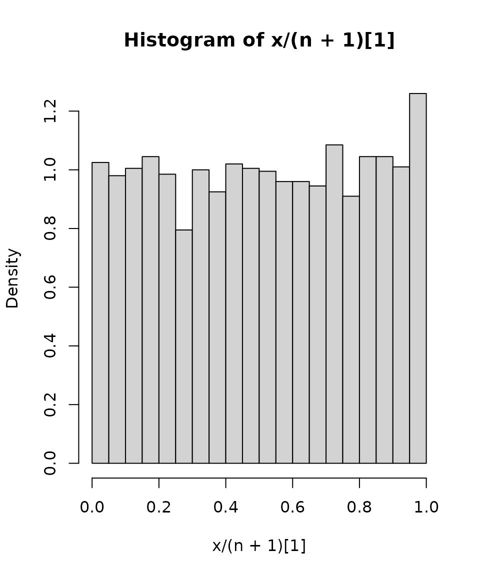
A histogram of the simulations of a random scalar x[1]}, can be plotted withrvhist}:

Example: Simulating P'olya’s Urn
This code simulates 200 iterations of the well-known P'olya’s urn problem. The parameter x/(n+1) for the Bernoulli-variate-generating function rvbern(...) is random: we can generate random variables using random parameters without much trickery; our code looks therefore more natural.
The model: \[\begin{eqnarray} \quad X_0 &= 1 \\ \quad X_n-X_{n-1}|X_{n-1} &\sim \text{Bernoulli}( X_{n-1}/(n+1) ) \end{eqnarray}\]
The R code:
  x <- 1
  for (n in 1:100) {
    x <- x + rvbern(n=1, prob=x / (n + 1))
  }
rvhist(x / (n + 1)) # Histogram
We can see that the distribution is close to uniform, which is the limiting distribution in this case.
Details
Obtaining the simulation matrix
To extract the simulation matrix embedded in an rv object, use sims:
It is our convention to have the columns represent the random vector and the rows represent the draws from the joint distribution of the vector.
Converting matrices and vectors of simulations to rv objects
A matrix or a vector of simulations is converted into an rv object by rvsims. Continuing the above example, we’ll convert the matrix back to an rv object.
y <- rvsims(s)You can verify that all(sims(y)==s) returns . % TRUE Also note that length(y) gives , since y is “just a vector.”
Coercing vectors and matrices
The function as.rv(x) coerces objects to rv objects. However, this does not mean that matrices of simulations are turned into rv objects—this is done with rvsims, as explained above. as.rv(rnorm(4000)) would return a random vector of length 4000, where each component has zero variance (and one single simulation). You probably mean rvsims(rnorm(4000)), but the correct way to generate this object is rvnorm(1).
Obtaining simulations from R2WinBUGS
R2WinBUGS (Sturtz, Ligges, and Gelman 2005) is an interface for calling WinBUGS within R, and obtaining the simulations as an R matrix (that is embedded in a “bugs” object). If bugsobj is the bugs object returned by the bugs(...) function call, then as.rv will coerce it into a list of random vectors, split by the parameter names: y <- as.rv(bugsobj)
Some implementation details
rv is written in “S3” style object-oriented R rather than using the methods (“S4”) package. The main reason was speed, the secondary consideration was the ease of writing new functions.
The main class is called rv. Most functions expecting an rv object have names starting with rv. For example, rvnorm, rvmean, etc.
The package also features rv-specific methods extending the basic numeric vector classes, e.g. c.rv, plot.rv, etc. However, the method dispatch in R will not call the rv class method if the first object in the argument list is not an rv object; for example, c(...) will not call c.rv in the following case: suppose that x is an object of class rv and k <- 10. Then c(k, x) will not call c.rv. To ensure the proper result, wrap the first element in as.rv:
c(as.rv(k), x) will produce a proper random vector.
Disclaimer
This program is a work in progress, and it may contain bugs. Many new features will be eventually (and hopefully) added.
For information about random variables in R, please refer to Kerman and Gelman (2007). For information about Umacs (Universal Markov chain sampler) please refer to Kerman (2005).
References
Kerman, Jouni. 2005. “Umacs A Universal Markov Chain Sampler.”
Kerman, Jouni, and Andrew Gelman. 2007. “Manipulating and Summarizing Posterior Simulations Using Random Variable Objects.” Statistics and Computing 17 (3): 235–44.
Sturtz, Sibylle, Uwe Ligges, and Andew Gelman. 2005. “R2WinBUGS A Package for Running WinBUGS from R.” Journal of Statistical Software 12 (3): 1–16.