Generate predictions from models

Performs predictions (in the form of rv objects) from models based on given covariates.

rvpredict(object, ...)

# S3 method for lm
rvpredict(object, newdata, ...)

Arguments

object: An object representing a statistical model fit.
...: Arguments passed to and from other methods.
newdata: A data frame with new covariates to be used in the predictions. The column names of the data frame must match those in the model matrix (although order may be arbitrary). If omitted, the model matrix is used instead; the resulting predictions are then the replications of the data. Note: this can be an rv object to incorporate extra uncertainty into predictions.

Value

For the lm method, a vector as long as there are rows in the data frame newdata.

Details

The lm method generates predictions of the outcome variable. The posterior coefficient estimates (the "intercept" and the "betas") are estimated in a Bayesian framework by posterior(object); the coefficients are multiplied by newdata (if omitted, the model covariate matrix is used instead) to obtain the predicted model mean; lastly, the outcomes are predicted from the Normal sampling model, taking into account the sampling variability along with the uncertainty in the estimation of the standard deviation (`sigma').

The covariate matrix newdata can be an rv, representing additional uncertainty in the covariates.

Author

J Kerman

Examples


  ## Create some fake data
  n <- 10
  ## Some covariates
  set.seed(1)
  X <- data.frame(x1=rnorm(n, mean=0), x2=rpois(n, 10) - 10)
  y.mean <- (1.0 + 2.0 * X$x1 + 3.0 * X$x2)
  y <- rnorm(n, y.mean, sd=1.5) ## n random numbers
  D <- cbind(data.frame(y=y), X)
  ## Regression model fit
  obj <- lm(y ~ x1 + x2, data=D)
  ## Bayesian estimates
  posterior(obj)
#> $beta
#>            name mean   sd    1%  2.5%  25%  50% 75% 97.5% 99% sims
#> [1] (Intercept) 0.88 0.57 -0.53 -0.29 0.55 0.88 1.2   2.0 2.3 1000
#> [2]          x1 2.88 0.97  0.74  1.10 2.27 2.87 3.4   4.8 5.5 1000
#> [3]          x2 3.24 0.22  2.64  2.80 3.11 3.23 3.4   3.7 3.8 1000
#> 
#> $sigma
#>     mean   sd   1% 2.5% 25% 50% 75% 97.5% 99% sims
#> [1]  1.7 0.61 0.95    1 1.3 1.6   2   3.2 3.7 1000
#> 
  ## Replications
  y.rep <- rvpredict(obj)
  ## Predictions at the mean of the covariates
  X.pred <- data.frame(x1=mean(X$x1), x2=mean(X$x2))
  y.pred <- rvpredict(obj, newdata=X.pred)
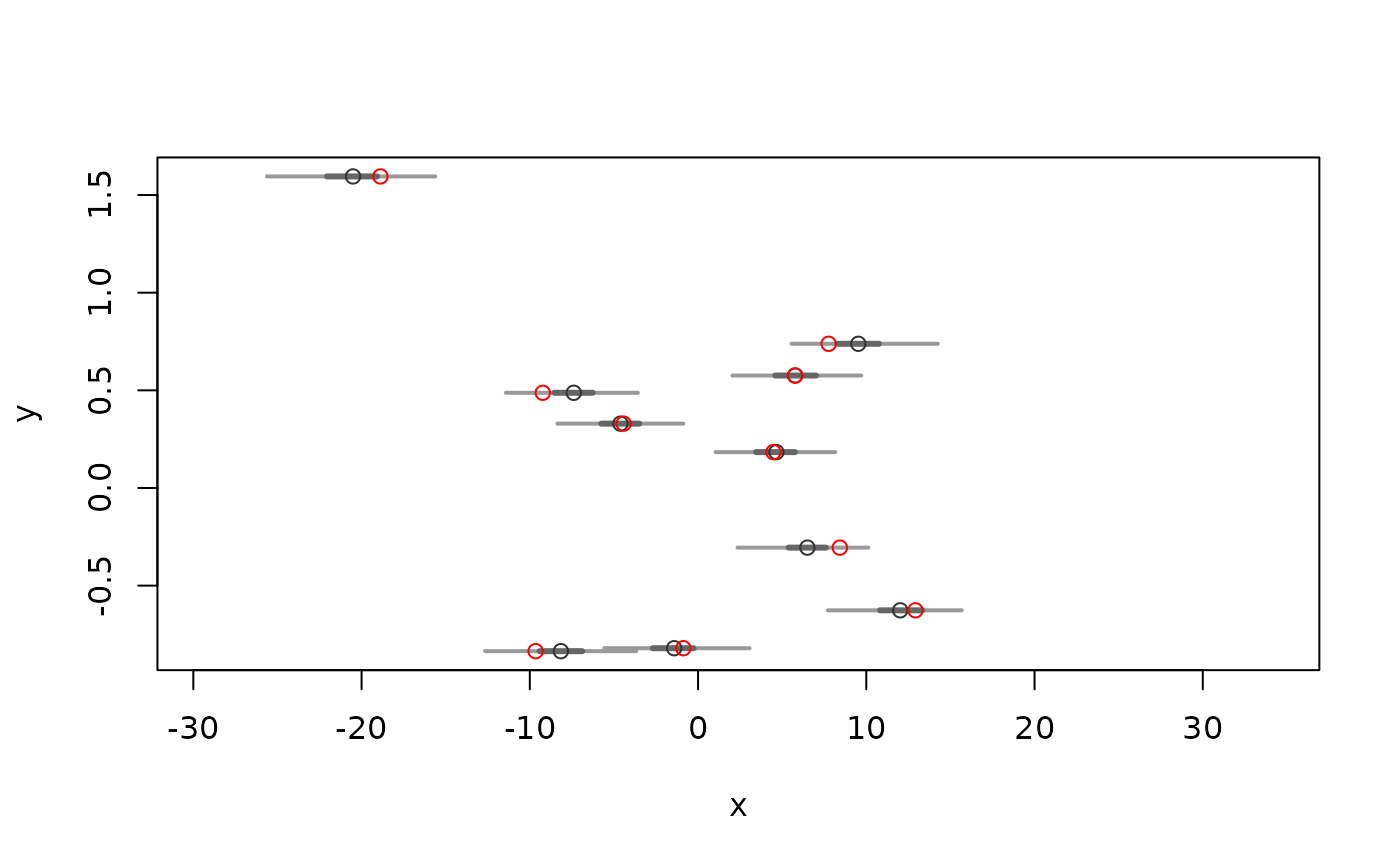
  ## Plot predictions
  plot(y.rep, D$x1)
  points(D$y, D$x1, col="red")

  ## 'Perturb' (add uncertainty to) covariate x1
  X.pred2 <- X
  X.pred2$x1 <- rnorm(n=n, mean=X.pred2$x1, sd=sd(X.pred2$x1))
  y.pred2 <- rvpredict(obj, newdata=X.pred2)