Manipulate Raster Data in R

Overview

Teaching: 40 min
Exercises: 20 min

Questions

• How can I crop raster objects to vector objects, and extract the summary of raster pixels?

Objectives

• Crop a raster to the extent of a vector layer.

• Extract values from a raster that correspond to a vector file overlay.

Things You’ll Need To Complete This Episode

See the lesson homepage for detailed information about the software, data, and other prerequisites you will need to work through the examples in this episode.

This episode explains how to crop a raster using the extent of a vector shapefile. We will also cover how to extract values from a raster that occur within a set of polygons, or in a buffer (surrounding) region around a set of points.

Crop a Raster to Vector Extent

We often work with spatial layers that have different spatial extents. The spatial extent of a shapefile or R spatial object represents the geographic “edge” or location that is the furthest north, south east and west. Thus is represents the overall geographic coverage of the spatial object.

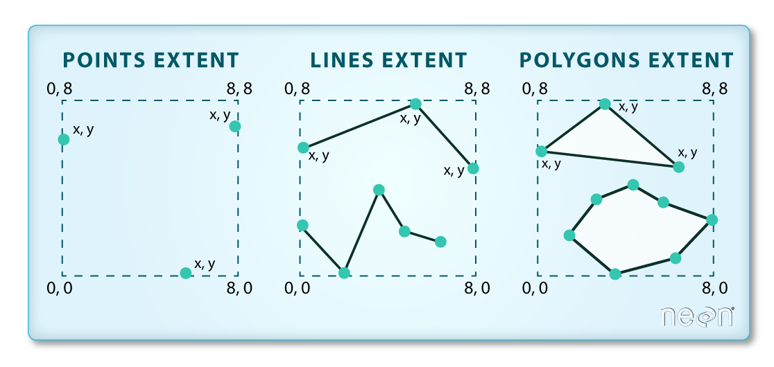Image Source: National Ecological Observatory Network (NEON)

The graphic below illustrates the extent of several of the spatial layers that we have worked with in this workshop:

• Lake erie outline (AOI) – blue
• Fish tracking locations (marked with white dots)– black
• An elevation surface in GeoTIFF format – green
• Walleye management zones – rainbow

Frequent use cases of cropping a raster file include reducing file size and creating maps. Sometimes we have a raster file that is much larger than our study area or area of interest. It is often more efficient to crop the raster to the extent of our study area to reduce file sizes as we process our data. Cropping a raster can also be useful when creating pretty maps so that the raster layer matches the extent of the desired vector layers.

Crop a Raster Using Vector Extent

We can use the crop() function to crop a raster to the extent of another spatial object. To do this, we need to specify the raster to be cropped and the spatial object that will be used to crop the raster. R will use the extent of the spatial object as the cropping boundary.

To illustrate this, we will crop the elevation surface to only include the area of interest (AOI). Let’s start by plotting the full extent of the elevation data and overlay where the AOI falls within it. The boundaries of the AOI will be colored blue, and we use fill = NA to make the area transparent.

ggplot() +
  geom_raster(data = erie_bathy_df, aes(x = x, y = y, fill = erie_bathy)) + 
  scale_fill_gradientn(name = "Bathymetry", colors = terrain.colors(10)) +
  geom_sf(data = erie_outline, color = "blue", fill = NA) +
  coord_sf()

Now that we have visualized the area of the elevation data we want to subset, we can perform the cropping operation. We are going to create a new object with only the portion of the elevation data that falls within the boundaries of the AOI. The function crop() is from the raster package and doesn’t know how to deal with sf objects. Therefore, we first need to convert erie_outline from a sf object to “Spatial” object.

erie_bathy_Cropped <- crop(x = erie_bathy, y = as_Spatial(erie_outline))

Now we can plot the cropped Lake Erie data, along with a boundary box showing the full elevation data extent. However, remember, since this is raster data, we need to convert to a data frame in order to plot using ggplot. To get the boundary box from Lake Erie, the st_bbox() will extract the 4 corners of the rectangle that encompass all the features contained in this object. The st_as_sfc() function converts these 4 coordinates into a polygon that we can plot:

erie_bathy_Cropped_df <- as.data.frame(erie_bathy_Cropped, xy = TRUE)

ggplot() +
  geom_sf(data = st_as_sfc(st_bbox(erie_bathy)), fill = "green",
          color = "green", alpha = .2) +  
  geom_raster(data = erie_bathy_Cropped_df,
              aes(x = x, y = y, fill = erie_bathy)) + 
  scale_fill_gradientn(name = "Bathymetry", colors = terrain.colors(10)) + 
  coord_sf()

The plot above shows that the full Lake Erie extent (plotted in green) is much larger than the resulting cropped raster. Our new cropped Lake Erie now has the same extent as the erie_outline object that was used as a crop extent (blue border below).

ggplot() +
  geom_raster(data = erie_bathy_Cropped_df,
              aes(x = x, y = y, fill = erie_bathy)) + 
  geom_sf(data = erie_outline, color = "blue", fill = NA) + 
  scale_fill_gradientn(name = "Bathymetry", colors = terrain.colors(10)) + 
  coord_sf()

We can look at the extent of all of our other objects we have to work with here.

st_bbox(erie_bathy)

   xmin    ymin    xmax    ymax 
 245701 4536578  754369 4767088 

st_bbox(erie_bathy_Cropped)

   xmin    ymin    xmax    ymax 
 285721 4580238  682057 4753028 

st_bbox(erie_outline)

     xmin      ymin      xmax      ymax 
 285728.3 4580281.1  682178.4 4752964.4 

st_bbox(fish_locations)

     xmin      ymin      xmax      ymax 
 319537.0 4609584.5  439213.4 4679545.8 

It would be nice to see our fishing tracking locations plotted on top of the Bathymetry information.

Challenge: Crop to Vector Points Extent

1. Crop the Bathymetry surface to the extent of the fish tracking locations.
2. Plot the fish tracking location points on top of the Bathymetry surface.

Answers

erie_bathy_crop <- crop(x = erie_bathy, y = as(fish_locations, "Spatial"))

erie_bathy_crop_df <- as.data.frame(erie_bathy_crop, xy = TRUE)

ggplot() + 
  geom_raster(data = erie_bathy_crop_df, aes(x = x, y = y, fill = erie_bathy)) + 
  scale_fill_gradientn(name = "Bathymetry", colors = terrain.colors(10)) + 
  geom_sf(data = fish_locations) + 
  coord_sf()

Define an Extent

So far, we have used a shapefile to crop the extent of a raster dataset. Alternatively, we can also the extent() function to define an extent to be used as a cropping boundary. This creates a new object of class extent. Here we will provide the extent() function our xmin, xmax, ymin, and ymax (in that order).

new_extent <- extent(285729, 385729, 4580282, 4752964)
class(new_extent)

[1] "Extent"
attr(,"package")
[1] "raster"

Data Tip

The extent can be created from a numeric vector (as shown above), a matrix, or a list. For more details see the extent() function help file (?raster::extent).

Once we have defined our new extent, we can use the crop() function to crop our raster to this extent object.

erie_bathy_manual_cropped <- crop(x = erie_bathy, y = new_extent)

To plot this data using ggplot() we need to convert it to a dataframe.

erie_bathy_manual_cropped_df <- as.data.frame(erie_bathy_manual_cropped, 
                                                xy = TRUE)

Now we can plot this cropped data. We will show the AOI boundary on the same plot for scale.

ggplot() + 
  geom_raster(data = erie_bathy_manual_cropped_df,
              aes(x = x, y = y, fill = erie_bathy)) + 
  scale_fill_gradientn(name = "Bathymetry", colors = terrain.colors(10)) + 
  geom_sf(data = erie_outline, color = "blue", fill = NA) +
  coord_sf()

Extract Raster Pixels Values Using Vector Polygons

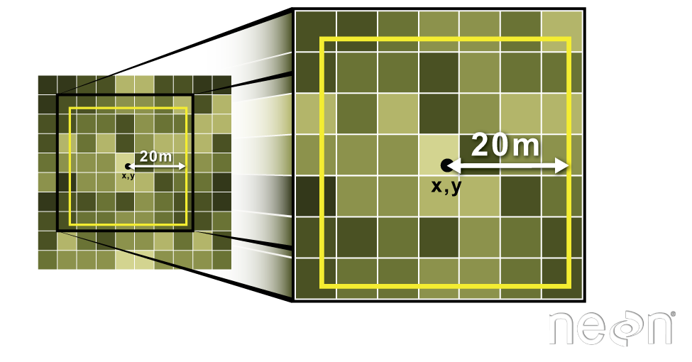
Often we want to extract values from a raster layer for particular locations - for example, our fish tracking locations that we are sampling. We can extract all pixel values within 20m of our x,y point of interest. These can then be summarized into some value of interest (e.g. mean, maximum, total).

To do this in R, we use the extract() function. The extract() function requires:

• The raster that we wish to extract values from,
• The vector layer containing the polygons that we wish to use as a boundary or boundaries,
• we can tell it to store the output values in a data frame using df = TRUE. (This is optional, the default is to return a list, NOT a data frame.) .

We will begin by extracting all bathymetry pixel values for our fish tracking locations.

fish_tracks_bathy <- extract(x = erie_bathy,
                       y = as(fish_locations, "Spatial"),
                       df = TRUE)

str(fish_tracks_bathy)

'data.frame':	1366 obs. of  2 variables:
 $ ID        : num  1 2 3 4 5 6 7 8 9 10 ...
 $ erie_bathy: num  -5.84 -4.42 -5.84 -4.83 -5.84 ...

When we use the extract() function, R extracts the value for each pixel located within the boundary of the polygon being used to perform the extraction - in this case the fish_locations object (a point layer). Here, the function extracted values from 1,366 pixels.

We can create a histogram of depth values within the boundary to better understand the structure or depth distribution at our fish tracking locations. We will use the column erie_bathy from our data frame as our x values, as this column represents the depths for each pixel.

ggplot() + 
  geom_histogram(data = fish_tracks_bathy, aes(x = erie_bathy)) +
  ggtitle("Histogram of Bathymetry Values (m)") +
  xlab("Depth") + 
  ylab("Frequency of Pixels")

`stat_bin()` using `bins = 30`. Pick better value with `binwidth`.

We can also use the summary() function to view descriptive statistics including min, max, and mean height values. These values help us better the depth at our fishing tracking locations.

summary(fish_tracks_bathy$erie_bathy)

   Min. 1st Qu.  Median    Mean 3rd Qu.    Max. 
-21.508 -13.786  -9.509 -10.177  -7.281   2.322 

Summarize Extracted Raster Values

We often want to extract summary values from a raster. We can tell R the type of summary statistic we are interested in using the fun = argument. Let’s extract a mean height value for our AOI. Because we are extracting only a single number, we will not use the df = TRUE argument.

mean_erie_bathy_AOI <- raster::extract(x = erie_bathy,
                              y = as(erie_outline, "Spatial"),
                              fun = mean)

mean_erie_bathy_AOI

          [,1]
[1,] -17.93646

It appears that the mean depth value, extracted from our bathymetry model is -17.9364625 meters.

Extract Data using x,y Locations

We can also extract pixel values from a raster by defining a buffer or area surrounding individual point locations using the extract() function. To do this we define the summary argument (fun = mean) and the buffer distance (buffer = 20) which represents the radius of a circular region around each point. By default, the units of the buffer are the same units as the data’s CRS. All pixels that are touched by the buffer region are included in the extract.

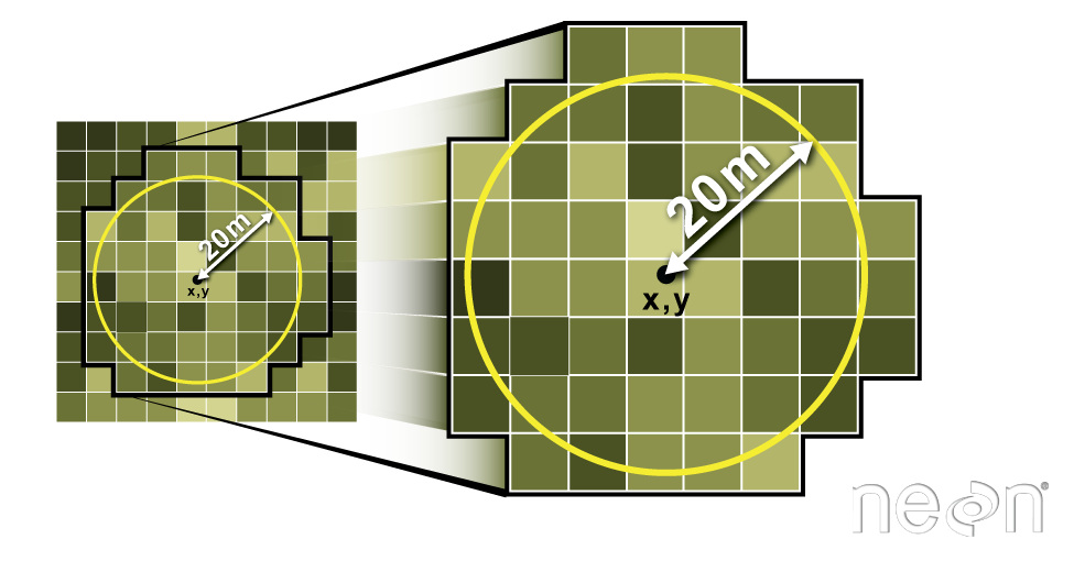
Source: National Ecological Observatory Network (NEON).

Let’s put this into practice by figuring out the mean depth in the 20m around the first fish tracking location (fish_locations). Because we are extracting from a single location, we will not use the df = TRUE argument.

mean_erie_fish <- extract(x = erie_bathy,
                           y = as(fish_locations[1,], "Spatial"),
                           fun = mean, buffer = 20)

mean_erie_fish

[1] -5.841959

Challenge: Extract buffered bathymetry values for fish tracking location

1) Use the fish tracking object (fish_locations) to extract an average depth for the area within 20m of each point location. Because there are multiple fish tracking locations, there will be multiple averages returned, so the df = TRUE argument should be used.

2) Create a plot showing the mean depth of each area.

Answers

# extract data at each fish tracking location
# mean_erie_fish_all <- extract(x = erie_bathy,
#                                y = as(fish_locations, "Spatial"),
#                               buffer = 20,
#                               fun = mean,
#                               df = TRUE)

# view data
# mean_erie_fish_all

# plot data
# ggplot(data = mean_erie_fish_all, aes(ID, erie_bathy)) + 
#  geom_col() + 
#  ggtitle("Mean Depth around each location") + 
#  xlab("ID") + 
#  ylab("Depth (m)")

Key Points

• Use the crop() function to crop a raster object.

• Use the extract() function to extract pixels from a raster object that fall within a particular extent boundary.

• Use the extent() function to define an extent.