Open and Plot Shapefiles in R

Overview

Teaching: 20 min
Exercises: 10 min

Questions

• How can I distinguish between and visualize point, line and polygon vector data?

Objectives

• Know the difference between point, line, and polygon vector elements.

• Load point, line, and polygon shapefiles into R.

• Access the attributes of a spatial object in R.

Things You’ll Need To Complete This Episode

See the lesson homepage for detailed information about the software, data, and other prerequisites you will need to work through the examples in this episode.

In this episode, we will introduce the fundamental principles, packages and metadata attributes that are needed to work with vector data in R. We will open and plot point, line and polygon vector data stored in shapefile format in R. In later episodes, we will learn how to work with raster and vector data together and combine them into a single plot.

Import Shapefiles

We will use the sf package to work with vector data in R. Notice that the rgdal package automatically loads when sf is loaded. We will also use the raster package, which we will work with in more detail in later episodes, so we can explore raster and vector spatial metadata using similar commands. Make sure you have the sf library loaded.

library(sf)

The shapefiles that we will import are:

• A polygon shapefile representing the outline of Lake Erie
• A line shapefile representing bathymetry contours

The first shapefile that we will open contains the outline of Lake Erie. To import shapefiles we use the sf function st_read(). st_read() requires the file path to the shapefile.

Let’s import our outline:

erie_outline <- st_read(
  "data/erie_outline.shp")

Reading layer `erie_outline' from data source `/home/jose/Documents/Science/Workshops/2020-02_glatos/glatos-spatial_workshop_materials/_episodes_rmd/data/erie_outline.shp' using driver `ESRI Shapefile'
Simple feature collection with 1 feature and 7 fields
geometry type:  POLYGON
dimension:      XY
bbox:           xmin: 285728.3 ymin: 4580281 xmax: 682178.4 ymax: 4752964
epsg (SRID):    NA
proj4string:    +proj=utm +zone=17 +ellps=GRS80 +units=m +no_defs

Shapefile Metadata & Attributes

When we import the Lake_Erie_Shoreline shapefile layer into R (as our erie_outline object), the st_read() function automatically stores information about the data. We are particularly interested in the geospatial metadata, describing the format, CRS, extent, and other components of the vector data, and the attributes which describe properties associated with each individual vector object.

Data Tip

The Explore and Plot by Shapefile Attributes episode provides more information on both metadata and attributes and using attributes to subset and plot data.

Spatial Metadata

Key metadata for all shapefiles include:

1. Object Type: the class of the imported object.
2. Coordinate Reference System (CRS): the projection of the data.
3. Extent: the spatial extent (i.e. geographic area that the shapefile covers) of the shapefile. Note that the spatial extent for a shapefile represents the combined extent for all spatial objects in the shapefile.

We can view shapefile metadata using the st_geometry_type(), st_crs() and st_bbox() functions. First, let’s view the geometry type for our outline shapefile:

st_geometry_type(erie_outline)

[1] POLYGON
18 Levels: GEOMETRY POINT LINESTRING POLYGON MULTIPOINT ... TRIANGLE

Our erie_outline is a polygon object. The 18 levels shown below our output list the possible categories of the geometry type. Now let’s check what CRS this file data is in:

st_crs(erie_outline)

Coordinate Reference System:
  No EPSG code
  proj4string: "+proj=utm +zone=17 +ellps=GRS80 +units=m +no_defs"

Our data in the CRS UTM zone 17N. The CRS is critical to interpreting the object’s extent values as it specifies units. To find the extent of our outline, we can use the st_bbox() function:

st_bbox(erie_outline)

     xmin      ymin      xmax      ymax 
 285728.3 4580281.1  682178.4 4752964.4 

The spatial extent of a shapefile or R spatial object represents the geographic “edge” or location that is the furthest north, south east and west. Thus is represents the overall geographic coverage of the spatial object.

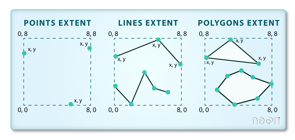Image Source: National Ecological Observatory Network (NEON).

Lastly, we can view all of the metadata and attributes for this shapefile object by printing it to the screen:

erie_outline

Simple feature collection with 1 feature and 7 fields
geometry type:  POLYGON
dimension:      XY
bbox:           xmin: 285728.3 ymin: 4580281 xmax: 682178.4 ymax: 4752964
epsg (SRID):    NA
proj4string:    +proj=utm +zone=17 +ellps=GRS80 +units=m +no_defs
  OBJECTID PERIMETER LAKE_NAME ID ReferenceC  ShapeSTAre ShapeSTLen
1        1   2445211 Lake Erie  1   60402132 25830205908    2445211
                        geometry
1 POLYGON ((643010.3 4749291,...

Spatial Data Attributes

Now we will explore how to use spatial data attributes stored in our data to plot different features.

Plot a Shapefile

Let’s visualize the data in our sf object using the ggplot package. Unlike with raster data, we do not need to convert vector data to a dataframe before plotting with ggplot.

We’re going to customize our boundary plot by setting the size, color, and fill for our plot. When plotting sf objects with ggplot2, you do not need to use the coord_sf() coordinate system.

library(ggplot2)

ggplot() + 
  geom_sf(data = erie_outline, size = 1.5, color = "black", fill = "cyan1") + 
  ggtitle("Lake Erie Outline") + 
  coord_sf()

Challenge: Import Line and Point Shapefiles

Using the steps above, import the erie_contours layer into R. Call the object erie_contours.

Answer the following questions:

1. What type of R spatial object is created when you import the layer?

2. What is the CRS and extent of the object?

3. Does the file contain points, lines, or polygons?

4. How many spatial objects are in the file?

Answers

First we import the data:

erie_contours <- st_read("data/erie_contours.shp")

Reading layer `erie_contours' from data source `/home/jose/Documents/Science/Workshops/2020-02_glatos/glatos-spatial_workshop_materials/_episodes_rmd/data/erie_contours.shp' using driver `ESRI Shapefile'
Simple feature collection with 8764 features and 3 fields
geometry type:  LINESTRING
dimension:      XY
bbox:           xmin: -83.57167 ymin: 41.36359 xmax: -78.7695 ymax: 42.9103
epsg (SRID):    4326
proj4string:    +proj=longlat +datum=WGS84 +no_defs

Then we check its class:

class(erie_contours)

[1] "sf"         "data.frame"

We also check the CRS and extent of the object:

st_crs(erie_contours)

Coordinate Reference System:
  EPSG: 4326 
  proj4string: "+proj=longlat +datum=WGS84 +no_defs"

st_bbox(erie_contours)

     xmin      ymin      xmax      ymax 
-83.57167  41.36359 -78.76950  42.91030 

To see the number of objects in the file, we can look at the output from when we read these objects into R. erie_contours contains 8764 features (all lines).

Key Points

• Shapefile metadata include geometry type, CRS, and extent.

• Load spatial objects into R with the st_read() function.

• Spatial objects can be plotted directly with ggplot using the geom_sf() function. No need to convert to a dataframe.