Seasonal and Regional Kendall trend test

Calculates the Seasonal or Regional Kendall test of trend significance, including an estimate of the Sen slope.

seaKen(
  x,
  plot = FALSE,
  type = c("slope", "relative"),
  order = FALSE,
  pval = 0.05,
  mval = 0.5,
  pchs = c(19, 21),
  ...
)

Arguments

x: A numeric vector, matrix or data frame made up of seasonal time series
plot: Should the trends be plotted when x is a matrix or data frame?
type: Type of trend to be plotted, actual or relative to series median
order: Should the plotted trends be ordered by size?
pval: p-value for significance
mval: Minimum fraction of seasons needed with non-missing slope estimates
pchs: Plot symbols for significant and not significant trend estimates, respectively
...: Other arguments to pass to plotting function

Value

A list of the following if x is a vector: seaKen

returns a list with the following members:

sen.slope: Sen slope
sen.slope.pct: Sen slope as percent of mean
p.value: significance of slope
miss: for each season, the fraction missing of slopes connecting first and last 20% of the years

or a matrix with corresponding columns if x is a matrix or data frame.

Details

The Seasonal Kendall test (Hirsch et al. 1982) is based on the Mann-Kendall tests for the individual seasons (see mannKen for additional details). p-values provided here are not corrected for serial correlation among seasons.

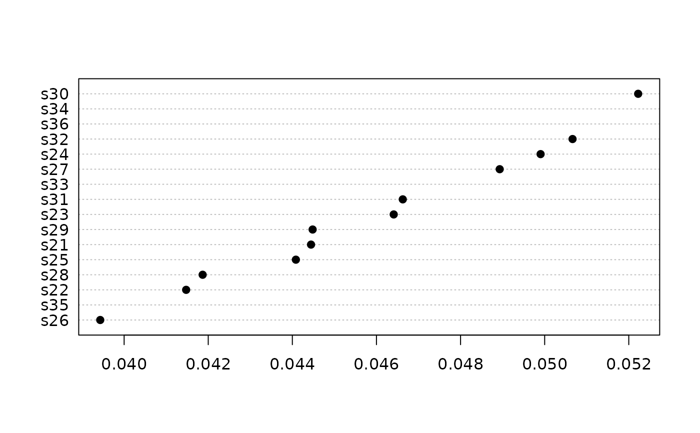
If plot = TRUE, then either the Sen slope in units per year (type = "slope") or the relative slope in fraction per year (type = "relative") is plotted. The relative slope is defined identically to the Sen slope except that each slope is divided by the first of the two values that describe the slope. Plotting the relative slope is useful when the variables in x are always positive and have different units.

The plot symbols indicate, respectively, that the trend is statistically significant or not. The plot can be customized by passing any arguments used by dotchart such as xlab, as well as graphical parameters described in par.

If mval or more of the seasonal slope estimates are missing, then that trend is considered to be missing. The seasonal slope estimate (mannKen), in turn, is missing if half or more of the possible comparisons between the first and last 20% of the years are missing.

The function can be used in conjunction with mts2ts to calculate a Regional Kendall test of significance for annualized data, along with a regional estimate of trend (Helsel and Frans 2006). See the examples below.

References

Helsel, D.R. and Frans, L. (2006) Regional Kendall test for trend. Environmental Science and Technology 40(13), 4066-4073.

Hirsch, R.M., Slack, J.R., and Smith, R.A. (1982) Techniques of trend analysis for monthly water quality data. Water Resources Research 18, 107-121.

Author

Alan Jassby, James Cloern

Examples


# Seasonal Kendall test:
chl <- sfbayChla # monthly chlorophyll at 16 stations in San Francisco Bay
seaKen(sfbayChla[, 's27']) # results for a single series at station 27
#> $sen.slope
#> [1] 0.1083333
#> 
#> $sen.slope.rel
#> [1] 0.04893086
#> 
#> $p.value
#> [1] 1.117981e-25
#> 
#> $miss
#> [1] 0.083
#> 
seaKen(sfbayChla) # results for all stations
#>      sen.slope sen.slope.rel      p.value  miss
#> s21 0.09672840    0.04444444 9.258533e-25 0.167
#> s22 0.08700000    0.04147465 1.837197e-20 0.167
#> s23 0.09925824    0.04641062 2.285817e-22 0.083
#> s24 0.09682540    0.04990329 1.651685e-29 0.083
#> s25 0.09500000    0.04408397 6.192363e-22 0.083
#> s26 0.09744390    0.03943167 2.147676e-16 0.083
#> s27 0.10833333    0.04893086 1.117981e-25 0.083
#> s28 0.09945682    0.04186706 7.150618e-16 0.167
#> s29 0.10600000    0.04448217 1.411127e-20 0.083
#> s30 0.12666667    0.05222332 2.743074e-24 0.083
#> s31 0.14021739    0.04662605 1.299337e-13 0.250
#> s32 0.15500000    0.05066313 8.497741e-19 0.167
#> s33 0.18761538    0.04847510 8.962505e-10 0.833
#> s34 0.18614815    0.05149382 1.285311e-12 0.833
#> s35 0.15965517    0.04040404 1.504345e-06 0.833
#> s36 0.18745098    0.05140187 1.231323e-11 0.833
seaKen(sfbayChla, plot=TRUE, type="relative", order=TRUE)


# Regional Kendall test:
# Use mts2ts to change 16 series into a single series with 16 "seasons"
seaKen(mts2ts(chl))  # too many missing data
#> $sen.slope
#> [1] 0.2440196
#> 
#> $sen.slope.rel
#> [1] 0.080248
#> 
#> $p.value
#> [1] 9.403823e-10
#> 
#> $miss
#> [1] 1
#> 
# better when just Feb-Apr, spring bloom period,
# but last 4 stations still missing too much.
seaKen(mts2ts(chl, seas = 2:4)) 
#> $sen.slope
#> [1] 0.2161335
#> 
#> $sen.slope.rel
#> [1] 0.04131365
#> 
#> $p.value
#> [1] 1.100025e-24
#> 
#> $miss
#> [1] 0.25
#> 
seaKen(mts2ts(chl[, 1:12], 2:4)) # more reliable result
#> $sen.slope
#> [1] 0.2155
#> 
#> $sen.slope.rel
#> [1] 0.04263112
#> 
#> $p.value
#> [1] 4.539847e-24
#> 
#> $miss
#> [1] 0
#>