Image plot of monthly time series

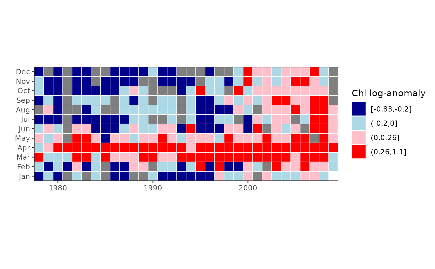
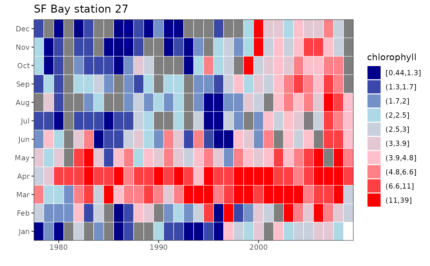
Monthly values are transformed into deciles or other bins, and corresponding colors are plotted in a month by year matrix.

plotTsTile(
  x,
  plot.title = NULL,
  legend.title = NULL,
  four = TRUE,
  loganom = TRUE,
  square = TRUE,
  legend = TRUE,
  trim = TRUE,
  overall = TRUE,
  stat = c("median", "mean")
)

Arguments

x

monthly time series.

plot.title

plot title.

legend.title

legend title.

four

logical indicating if data should be binned into 4 special groups or into deciles.

loganom

logical indicating if data should be transformed into log-anomalies.

square

logical indicating if tiles should be square.

legend

logical indicating if a legend should be included.

trim

logical indicating if leading and trailing NA values should be removed.

overall

determines whether anomalies are calculated with respect to overall mean or to long-term mean for the same month.

stat

determines whether anomalies are calculated and binned using mean or median.

Value

An image plot of monthly values classified into either deciles or into four bins as described above (and corresponding object of class “ggplot”).

Details

If four = TRUE, then x is first divided into a positive and negative bin. Each bin is then further divided into two bins by its mean, yielding a total of four bins. If four=FALSE, then x is simply divided into deciles. In either case, each bin has its own assigned color, with colors ranging from dark blue (smallest numbers) through light blue and pink to red.

Although four = TRUE can be useful for any data in which 0 represents a value with special significance, it is especially so for data converted into log-anomalies, i.e., log10(x/xbar) where xbar = mean(x, na.rm=TRUE). The mean month then has value 0, and a value of -1, for example, indicates original data equal to one-tenth the mean. Log-anomaly transforms can be particularly appropriate for biological populations, in which variability is often approximately proportional to the mean.

When loganom = TRUE, the anomalies are calculated with respect to the overall mean month. This differs from, for example, the log-anomaly zooplankton plot of O'Brien et al. (2008), in which a monthly anomaly is calculated with respect to the mean value of the same month. To get the latter behavior, set overall = FALSE. A further option is to set stat = "median" rather than the default stat = "mean", in which case xbar = median(x, na.rm = TRUE), and the positive and negative bins are each divided into two bins by their median instead of mean. Using combinations of these different options can reveal complementary information.

You may want to set square = FALSE and then adjust the plot window manually if you plan to use the plot in a subsequent layout or if there is too much white space.

References

O'Brien T., Lopez-Urrutia A., Wiebe P.H., Hay S. (editors) (2008) ICES Zooplankton Status Report 2006/2007. ICES Cooperative Research Report 292, International Council for the Exploration of the Sea, Copenhagen, 168 p.

Author

Alan Jassby, James Cloern

Examples

# plot log-anomalies in four bins
chl27 = sfbayChla[, 's27']
plotTsTile(chl27, legend.title = 'Chl log-anomaly')


# plot deciles
plotTsTile(chl27, plot.title = 'SF Bay station 27', legend.title =
  'chlorophyll', four = FALSE, loganom = FALSE, square = FALSE)