Calculate Kernel Density Using River Distance

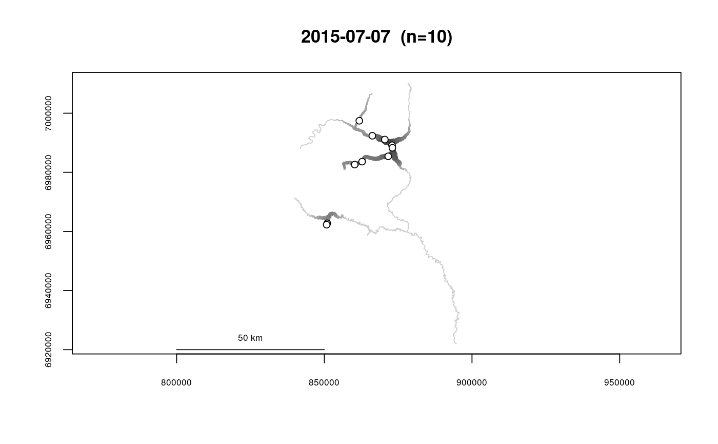
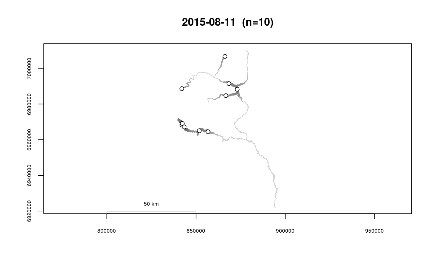
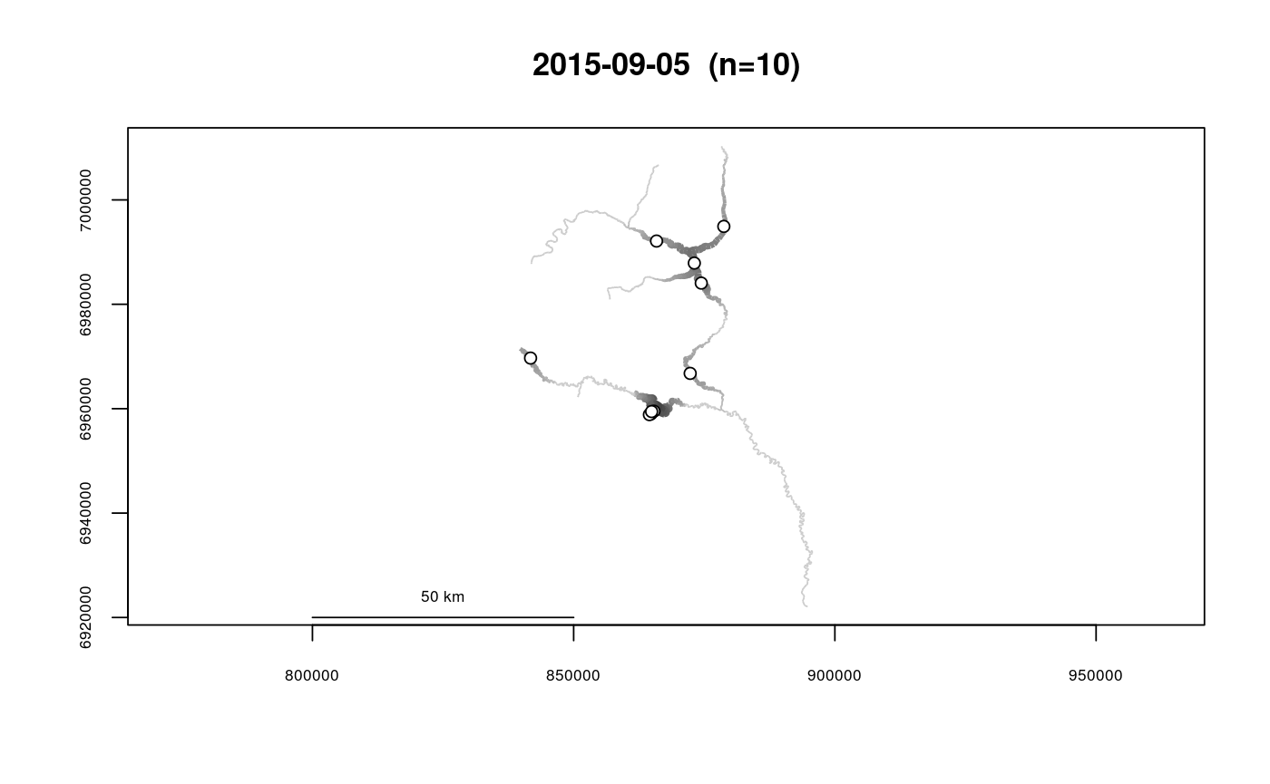
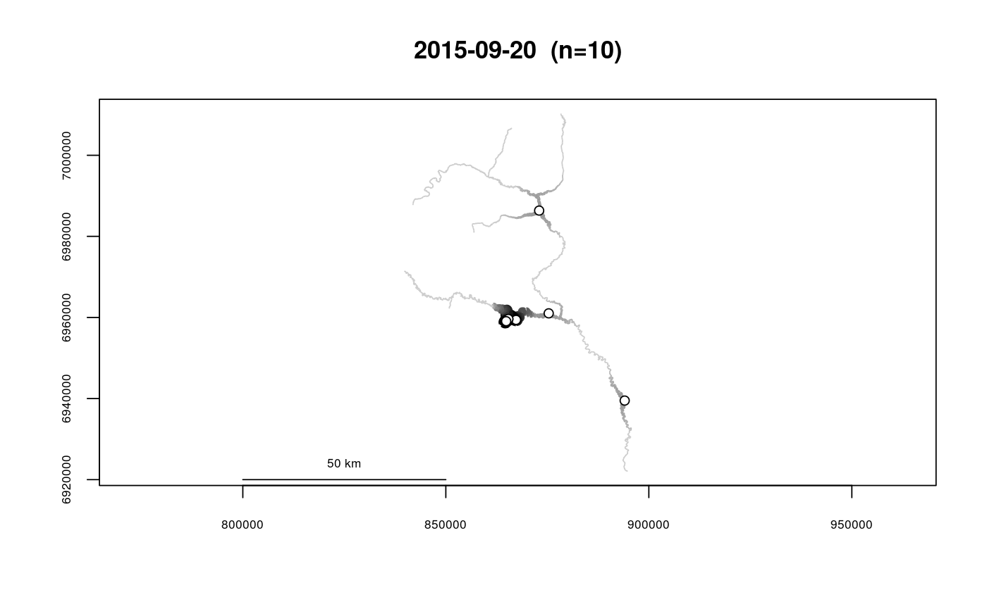
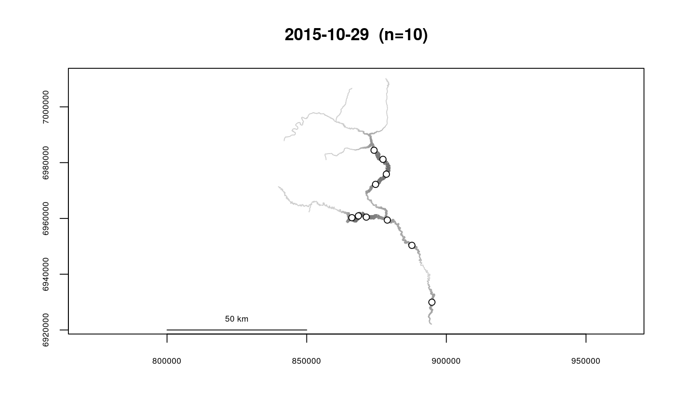
Uses spatial point data (segment and vertex) to calculate a kernel density object to use in the output class plotting method,plot.riverdensity. Scaled kernel density is calculated at approximately regularly-spaced locations, with spacing specified by the user.

If an argument is used in the survey field, kernel densities will be calculated for each unique value of survey, resulting in a separate plot for each.

The purpose of this function is to generate a kernel density object to plot using plot(), see plot.riverdensity.

makeriverdensity(seg, vert, rivers, survey = NULL, kernel = "gaussian",
  bw = NULL, resolution = NULL)

Arguments

seg	A vector of river locations (segment)
vert	A vector of river locations (vertex)
rivers	The river network object to use
survey	A vector of survey IDs corresponding to the values of seg and vert. If this argument is used, kernel densities will be calculated for each unique survey, and separate plots will be produced.
kernel	The type of density kernel to use. Allowed types are "gaussian" (normal) and "rect" (rectangular, giving simple density). Defaults to "gaussian".
bw	The kernel bandwidth to use. If kernel is set to "gaussian", this provides the standard deviation of the gaussian (normal) kernel to use. If kernel is set to "rect", this provides the half-width of the rectangular kernel, or the distance to use in simple density. Accepting the default (NULL) will result in the function determining a value to use, based on the total length of the river network and the value of the resolution argument.
resolution	The approximate spacing of the river locations used for kernel density calculation. Accepting the default (NULL) will result in the function determining a value to use, based on the total length of the river network.

Value

A river density object, see riverdensity-class.

Note

It is likely that calculation will be very slow. Use of this function with a river network for which segment routes has not yet been calculated is not recommended.

This function is distance-computation intensive, and may be slow-running if a river network is used that does not have segment routes and/or distance lookup tables for fast distance computation. See buildsegroutes and/or buildlookup for more information.

See also

plot.riverdensity, plotriverdensitypoints

Examples

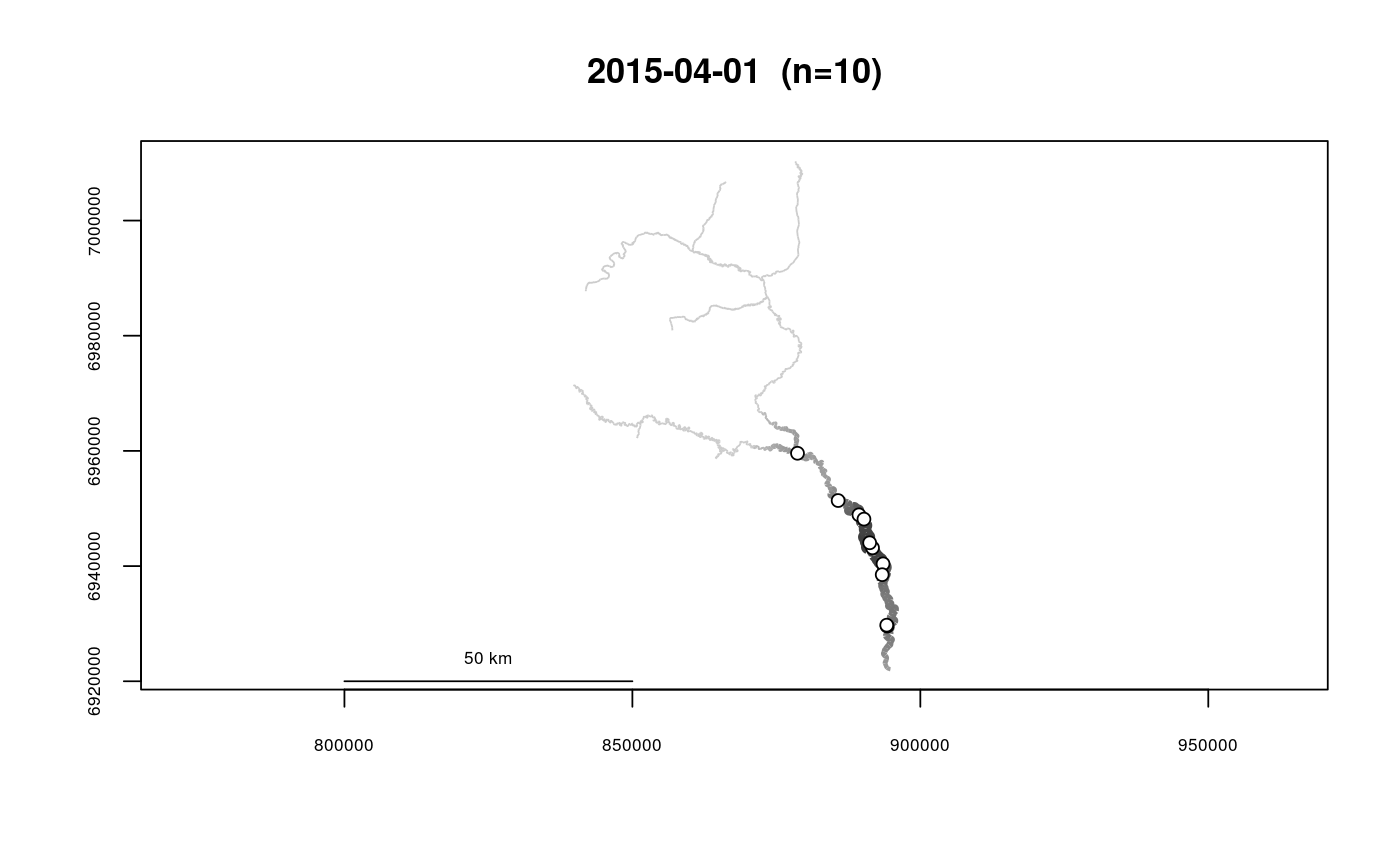
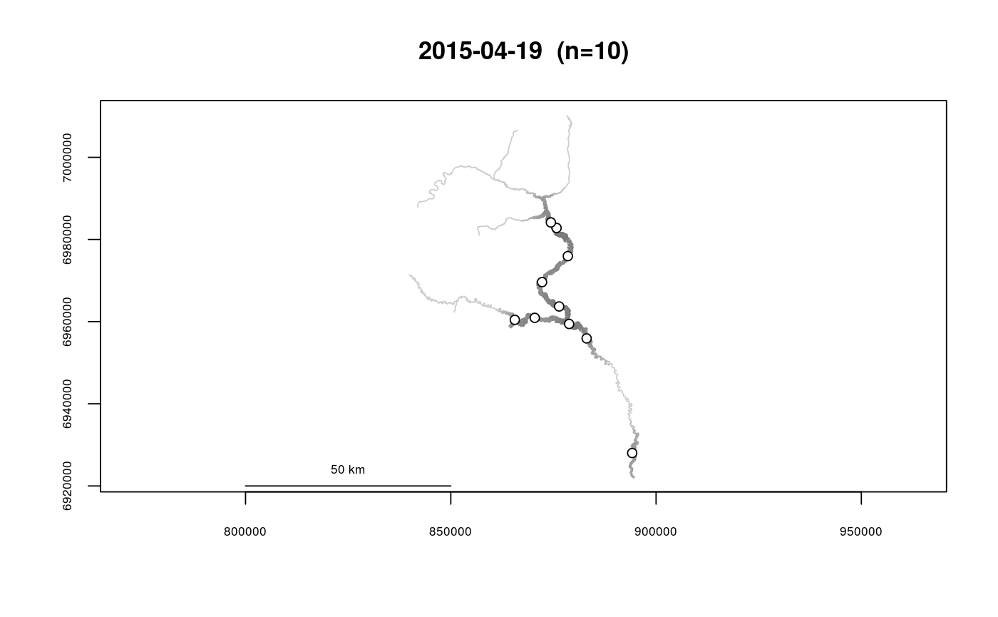
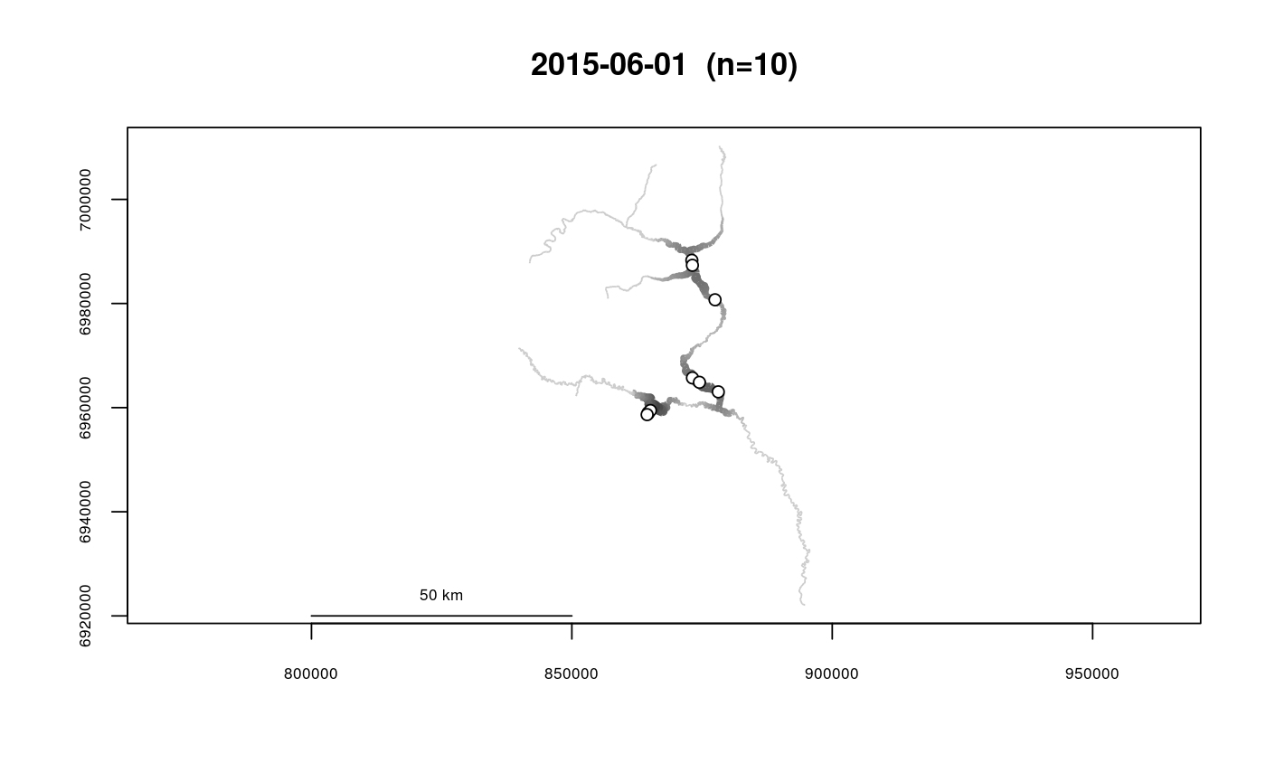
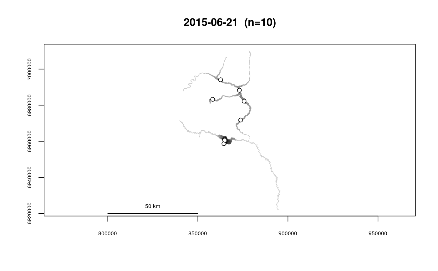
data(Gulk, fakefish)

Gulk_dens <- makeriverdensity(seg=fakefish$seg, vert=fakefish$vert, rivers=Gulk,
  survey=fakefish$flight.date)
#> 
  |                                                                            
  |                                                                      |   0%
  |                                                                            
  |                                                                      |   1%
  |                                                                            
  |=                                                                     |   1%
  |                                                                            
  |==                                                                    |   2%
  |                                                                            
  |==                                                                    |   3%
  |                                                                            
  |==                                                                    |   4%
  |                                                                            
  |===                                                                   |   4%
  |                                                                            
  |====                                                                  |   5%
  |                                                                            
  |====                                                                  |   6%
  |                                                                            
  |=====                                                                 |   6%
  |                                                                            
  |=====                                                                 |   7%
  |                                                                            
  |======                                                                |   8%
  |                                                                            
  |======                                                                |   9%
  |                                                                            
  |=======                                                               |  10%
  |                                                                            
  |========                                                              |  11%
  |                                                                            
  |========                                                              |  12%
  |                                                                            
  |=========                                                             |  13%
  |                                                                            
  |==========                                                            |  14%
  |                                                                            
  |===========                                                           |  15%
  |                                                                            
  |===========                                                           |  16%
  |                                                                            
  |============                                                          |  16%
  |                                                                            
  |============                                                          |  17%
  |                                                                            
  |============                                                          |  18%
  |                                                                            
  |=============                                                         |  19%
  |                                                                            
  |==============                                                        |  19%
  |                                                                            
  |==============                                                        |  20%
  |                                                                            
  |===============                                                       |  21%
  |                                                                            
  |================                                                      |  22%
  |                                                                            
  |================                                                      |  23%
  |                                                                            
  |================                                                      |  24%
  |                                                                            
  |=================                                                     |  24%
  |                                                                            
  |==================                                                    |  25%
  |                                                                            
  |==================                                                    |  26%
  |                                                                            
  |===================                                                   |  27%
  |                                                                            
  |====================                                                  |  28%
  |                                                                            
  |====================                                                  |  29%
  |                                                                            
  |=====================                                                 |  30%
  |                                                                            
  |=====================                                                 |  31%
  |                                                                            
  |======================                                                |  31%
  |                                                                            
  |======================                                                |  32%
  |                                                                            
  |=======================                                               |  33%
  |                                                                            
  |=======================                                               |  34%
  |                                                                            
  |========================                                              |  34%
  |                                                                            
  |========================                                              |  35%
  |                                                                            
  |=========================                                             |  36%
  |                                                                            
  |==========================                                            |  36%
  |                                                                            
  |==========================                                            |  37%
  |                                                                            
  |==========================                                            |  38%
  |                                                                            
  |===========================                                           |  39%
  |                                                                            
  |============================                                          |  39%
  |                                                                            
  |============================                                          |  40%
  |                                                                            
  |============================                                          |  41%
  |                                                                            
  |=============================                                         |  41%
  |                                                                            
  |==============================                                        |  42%
  |                                                                            
  |==============================                                        |  43%
  |                                                                            
  |==============================                                        |  44%
  |                                                                            
  |===============================                                       |  44%
  |                                                                            
  |================================                                      |  45%
  |                                                                            
  |================================                                      |  46%
  |                                                                            
  |=================================                                     |  47%
  |                                                                            
  |==================================                                    |  48%
  |                                                                            
  |==================================                                    |  49%
  |                                                                            
  |===================================                                   |  50%
  |                                                                            
  |====================================                                  |  51%
  |                                                                            
  |====================================                                  |  52%
  |                                                                            
  |=====================================                                 |  53%
  |                                                                            
  |======================================                                |  54%
  |                                                                            
  |======================================                                |  55%
  |                                                                            
  |=======================================                               |  56%
  |                                                                            
  |========================================                              |  56%
  |                                                                            
  |========================================                              |  57%
  |                                                                            
  |========================================                              |  58%
  |                                                                            
  |=========================================                             |  59%
  |                                                                            
  |==========================================                            |  59%
  |                                                                            
  |==========================================                            |  60%
  |                                                                            
  |==========================================                            |  61%
  |                                                                            
  |===========================================                           |  61%
  |                                                                            
  |============================================                          |  62%
  |                                                                            
  |============================================                          |  63%
  |                                                                            
  |============================================                          |  64%
  |                                                                            
  |=============================================                         |  64%
  |                                                                            
  |==============================================                        |  65%
  |                                                                            
  |==============================================                        |  66%
  |                                                                            
  |===============================================                       |  67%
  |                                                                            
  |================================================                      |  68%
  |                                                                            
  |================================================                      |  69%
  |                                                                            
  |=================================================                     |  70%
  |                                                                            
  |=================================================                     |  71%
  |                                                                            
  |==================================================                    |  71%
  |                                                                            
  |==================================================                    |  72%
  |                                                                            
  |===================================================                   |  73%
  |                                                                            
  |===================================================                   |  74%
  |                                                                            
  |====================================================                  |  74%
  |                                                                            
  |====================================================                  |  75%
  |                                                                            
  |=====================================================                 |  76%
  |                                                                            
  |======================================================                |  76%
  |                                                                            
  |======================================================                |  77%
  |                                                                            
  |======================================================                |  78%
  |                                                                            
  |=======================================================               |  79%
  |                                                                            
  |========================================================              |  79%
  |                                                                            
  |========================================================              |  80%
  |                                                                            
  |========================================================              |  81%
  |                                                                            
  |=========================================================             |  81%
  |                                                                            
  |==========================================================            |  82%
  |                                                                            
  |==========================================================            |  83%
  |                                                                            
  |==========================================================            |  84%
  |                                                                            
  |===========================================================           |  84%
  |                                                                            
  |============================================================          |  85%
  |                                                                            
  |============================================================          |  86%
  |                                                                            
  |=============================================================         |  87%
  |                                                                            
  |==============================================================        |  88%
  |                                                                            
  |==============================================================        |  89%
  |                                                                            
  |===============================================================       |  90%
  |                                                                            
  |================================================================      |  91%
  |                                                                            
  |================================================================      |  92%
  |                                                                            
  |=================================================================     |  93%
  |                                                                            
  |==================================================================    |  94%
  |                                                                            
  |==================================================================    |  95%
  |                                                                            
  |===================================================================   |  96%
  |                                                                            
  |====================================================================  |  96%
  |                                                                            
  |====================================================================  |  97%
  |                                                                            
  |====================================================================  |  98%
  |                                                                            
  |===================================================================== |  99%
  |                                                                            
  |======================================================================|  99%
  |                                                                            
  |======================================================================| 100%

# # 10 plots will be created, recommend calling par(mfrow=c(2,5))
plot(x=Gulk_dens)