Regression with Gibbs sampling
b.update <- function(y, sinv){
  if(length(sinv) == 1){
    sx <- crossprod(x) * sinv
    sy <- crossprod(x, y) * sinv
  }

  if(length(sinv) > 1){
    ss <- t(x) %*% sinv
    sx <- ss  %*% x
    sy <- ss %*% y
  }

  bigv   <- solve(sx + vinvert)
  smallv <- sy + vinvert %*% bprior
  b      <- t(rmvnorm(1, bigv %*% smallv, bigv))
  b
}

v.update <- function(y, rinverse){
  if(length(rinverse) == 1){
    sx <- crossprod((y - x %*% b))
  }
  if(length(rinverse) > 1){
    sx <- t(y - x %*% b) %*% rinverse %*% (y - x %*% b)
  }
  u1 <- s1 + 0.5 * n
  u2 <- s2 + 0.5 * sx

  1 / rgamma(1, u1, u2)
}
A nonlinear model
n     <- 100
light <- runif(n, 0, 1)                               # covariate vector
th0   <- 0.1                                          # theta
z     <- light / (th0 + light)
x     <- cbind(rep(1, n), z)                          # n by 2 design matrix

b0   <- 12                                            # regression parameters
b1   <- 40
beta <- matrix(c(b0, b1), 2, 1)
sig  <- 25
y    <- matrix(rnorm(n, x %*% beta, sqrt(sig)), n, 1) # response vector

# plot(x[,2], y)
ngibbs  <- 10000
thgibbs <- rep(0.1, ngibbs)
th      <- 0.1
x[,2]   <- light/(th + light)
bgibbs  <- matrix(0, nrow = ngibbs, ncol = 2)
sgibbs  <- rep(1, ngibbs)
sg      <- 1

thseq <- seq(0.05, 0.3, length = 100)
tmat  <- matrix(rep(thseq, each = n), nrow = n, byrow = FALSE)
lmat  <- matrix(rep(light, each = 100), nrow = n, byrow = TRUE)
zmat  <- lmat / (lmat + tmat)
ymat  <- matrix(rep(y, each = 100), nrow = n, byrow = TRUE)
bprior  <- as.vector(c(0, 0))
vinvert <- solve(diag(1000, 2))
ppart   <- vinvert %*% bprior
s1      <- 0.1
s2      <- 0.1
for(g in 1:ngibbs){
b <- b.update(y, 1 / sg)
sg <- v.update(y, 1)
mmat <- b[1] + b[2] * zmat
plik <- apply(dnorm(ymat, mmat, sqrt(sg), log = TRUE), 2, sum)
pseq <- exp(plik - max(plik))
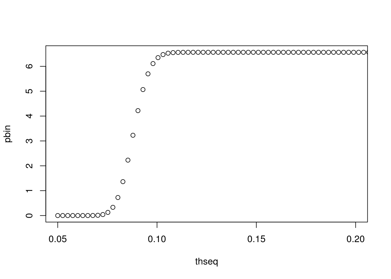
pbin <- cumsum(pseq)
zp <- runif(1, pbin[1], pbin[100])
thgibbs[b] <- thseq[findInterval(zp, pbin)]
x[,2] <- light / (th + light)
bgibbs[g,] <- b
sgibbs[g] <- sg
th <- thgibbs[g]
}
plot(thseq, pbin, xlim = c(0.05, 0.2))