Spatial Interpolation via Inverse Path Distance Weighting

J. Stachelek

2023-01-05

Abstract

The R package ipdw provides functions for interpolation of georeferenced point data via Inverse Path Distance Weighting. Useful for coastal marine applications where barriers in the landscape preclude interpolation with Euclidean distances. This method of interpolation requires significant computation and is only practical for relatively small and coarse grids. The ipdw implementation may provide additional flexibility and greater speed relative to alternatives.

Introduction

This vignette describes ipdw, an R package which provides the functionality to perform interpolation of georeferenced point data using inverse path distance weighting (Suominen, Tolvanen, and Kalliola 2010). Interpolation is accomplished in two steps. First, path distances are calculated from each georeferenced (measurement) point to each prediction point. Path distances, which honor barriers in the landscape, are calculated based on cell-to-cell movement through an underlying Raster object (Hijmans 2014) that represents movement cost. These path distances are subsequently used as interpolation weights. The two-step routine follows the order of operations described in Suominen, Tolvanen, and Kalliola (2010) substituting the ESRI path distance algorithm Mitchell (2012) with the gdistance (Etten 2014) wrapped version of the igraph (Csardi and Nepusz 2006) adjacency algorithm.

The ipdw package was developed with coastal marine applications in mind where path distances (as the fish swims) rather than Euclidean (as the crow flies) distances more accurately represent spatial connectivity (Little, Edwards, and Porter 1997). Interpolation of sparse grids in coastal areas otherwise end up bleeding through land areas (Stachelek and Madden 2015). The remainder of this vignette provides an example of such a situation using the Kattegat salinity dataset (Diggle and Lophaven 2006) found within the geoR package.

Data Preparation

library(ipdw)

To begin, we need to load an object representing point observations as either a matrix of coordinates or an sf object with point geometries and an object representing a coastline as an sf object with polygon geometries. The data for this demonstration come from a built-in dataset in the geoR package for the Kattegat basin of Denmark (see ?geoR::kattegat).

library(sf)
pols <- st_read(system.file("extdata/kattegat_coast.gpkg", package = "ipdw"))
pnts <- st_read(system.file("extdata/kattegat_pnts.gpkg", package = "ipdw"))

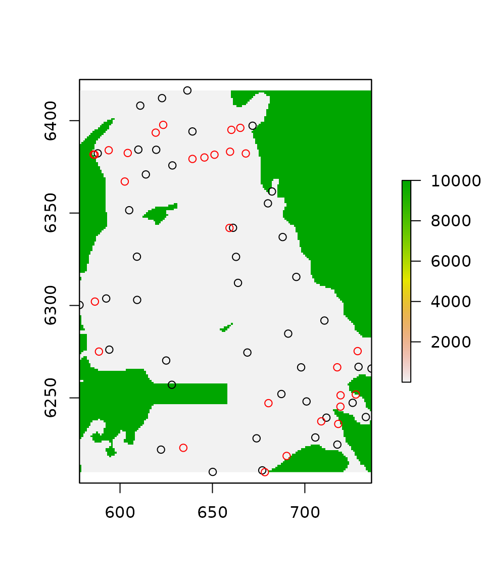
We can use this polygon sf object to create a cost raster defining travel through land areas with a very high cost. As a result, interpolation neighborhoods will be defined based on in-water rather than Euclidean distances. Cost raster creation is accomplished with the ipdw function costrasterGen. By default, open water areas are set to a per unit travel cost of 1 whereas land areas are set to a per unit travel cost of 10,000. Note that a projection is defined for the costrasterGen function by the projstr parameter. It is critical to check the resolution of the cost raster before proceeding. The resolution of the cost raster will determine the resolution of the interpolated output. If the resolution is too fine, this will result in very long processing times. If necessary, coarsen the cost raster with the raster function aggregate.

costras <- costrasterGen(pnts, pols, extent = "pnts",
  projstr = projection(pols))
# insert contiguous barrier
costras[160:170, 1:80] <- 10000

In order to evaluate the utility of IPDW, we split the dataset into separate training and validation datasets. The training dataset is created in a spatially balanced manner by building a grid and randomly selecting one measurement point per grid cell. In the following code block, the size of this grid is defined as 2 times the average distance among measurement points. Average distance is computed using the spatstat package (Baddeley and Turner 2005). Random selection is accomplished with the gdata function resample (Warnes et al. 2014). Subsetting the full dataset is not required to run ipdw. Alternative means of estimating interpolation errors, such as leave-one-out cross validation, are in development.

# find average nearest neighbor
library(spatstat)

W              <- owin(range(c(st_bbox(pnts)["xmin"], st_bbox(pnts)["xmax"])),
                       range(c(st_bbox(pnts)["ymin"], st_bbox(pnts)["ymax"])))
kat.pp         <- ppp(st_coordinates(pnts)[,1], st_coordinates(pnts)[,2], window = W)
mean.neighdist <- mean(nndist(kat.pp))

# grid building
gridsize       <- mean.neighdist * 2
grainscale.fac <- gridsize / res(costras)[1]
gridras        <- aggregate(costras, fact = grainscale.fac)
gridpol        <- rasterToPolygons(gridras)
gridpol$value  <- row.names(gridpol)

# spatial join
fulldataset.over <- sf::st_join(pnts, st_as_sf(gridpol))

# grid selection
set.seed(2)
gridlev <- unique(fulldataset.over$value)
for (i in seq_along(gridlev)) {
  activesub <- subset(fulldataset.over, fulldataset.over$value == gridlev[i])
  selectnum <- gdata::resample(seq_len(nrow(activesub)), 1)
  if (i == 1) {
    training <- activesub[selectnum, ]
  } else {
    training <- rbind(training, activesub[selectnum, ])
  }
}

Next, we save the training and validation datasets as objects of class class sf with point geometries. Note that the projection of the training and validation datasets matches the cost raster we created previously. Calculations within the ipdw package require projected datasets. More about R projections can be found from the PROJ.4 documentation at the Open Source Geospatial Foundation (https://proj4.org).

validate             <- fulldataset.over[!(row.names(fulldataset.over) %in%
  row.names(training)), ]

plot(costras)
plot(st_geometry(training), add = TRUE)
plot(st_geometry(validate), col = "red", add = TRUE)

Figure 1: Cost raster representing the high cost of travel through land areas. Training and validation points are shown in black and red respectively.

Interpolation

We have assembled an object of class sf with point geometries to be interpolated and an underlying cost raster of class Raster. We can either proceed in a single step using the high-level ipdw function ipdw or in two steps using calls to the pathdistGen and ipdwInterp functions. For simplicity, the single step option, ipdw, is shown below. The two step option would be useful for the case where we want interpolate multiple parameters of the same sf object using a single RasterStack of path distances.

paramlist <- c("salinity")
final.ipdw <- ipdw(training, costras, range = mean.neighdist * 10, paramlist,
  overlapped = TRUE)

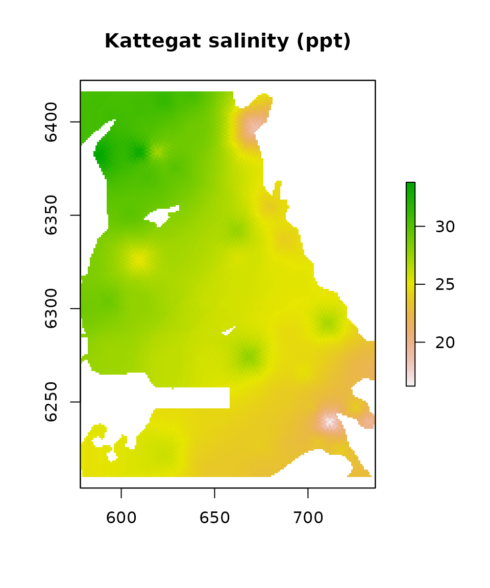
plot(final.ipdw, main = "Kattegat salinity (ppt)")

Figure 2: Interpolated salinity surface by IPDW.

Comparison with Inverse Distance Weighting

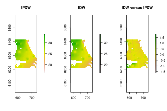
We can evaluate the benefits of IPDW by comparing its output against Inverse Distance Weighting with Euclidean distances. The following section generates an interpolated surface via IDW. First, prediction points are generated. Then the gstat (Pebesma 2004) IDW functionality is called with the same inputs as the previous section above. Differences between the outputs of two methodologies are shown in Figure 2.

idw.grid <- rasterToPoints(costras, fun = function(x) {
  x < 10000
}, spatial = FALSE)
idw.grid <- st_as_sf(data.frame(idw.grid), coords = c("x", "y"), crs = st_crs(training))
kat.idw  <- gstat::idw(salinity ~ 1, training, idw.grid, maxdist = mean.neighdist * 10,
  debug.level = 0)["var1.pred"]
final.idw <- rasterize(as_Spatial(kat.idw), final.ipdw)
final.idw <- raster::subset(final.idw, "var1.pred")

par(mfrow = c(1, 3), mar = c(5.1, 4.1, 4.1, 5.1))
plot(final.ipdw, main = "IPDW")
plot(final.idw, main = "IDW")
plot(final.idw - final.ipdw,  main = "IDW versus IPDW")

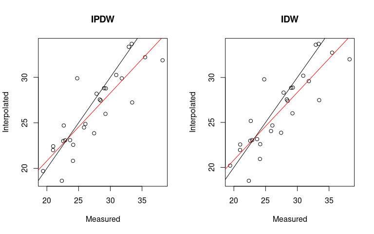
We can compare interpolation errors quantitatively using the errorGen function. Figure 3 shows a plot of the validation dataset against the interpolated estimates at those points. The validation dataset enters into the function both as a sf object and as the underlying data values.

measured.spdf              <- data.frame(validate$salinity)

valid.ipdw <- errorGen(final.ipdw, validate["salinity"], measured.spdf)
valid.idw  <- errorGen(final.idw, validate["salinity"], measured.spdf)

par(mfrow = c(1, 2))
valid.ipdw <- errorGen(final.ipdw, validate["salinity"], measured.spdf,
  plot = TRUE, title = "IPDW")
valid.idw <- errorGen(final.idw, validate["salinity"], measured.spdf,
  plot = TRUE, title = "IDW")

Results from IDW and IPDW appear similar because no validation points are present in the area downstream (south) of the contiguous barrier (Figure 1, 2). Up to this point, we have seen a simple implementation of IPDW requiring only an sf object with point geometries and a cost Raster.

Test comparisons between the ipdw and the ESRI (Mitchell 2012; Suominen, Tolvanen, and Kalliola 2010) implementations of IPDW found ipdw to be much faster and more flexible. In particular, the high-level function ipdw provides the ability to run IPDW in one step while the lower-level function ipdwInterp can be called multiple times following pathdistGen in order to interpolate multiple parameters of a single sf object. This is accomplished by saving the output from pathdistGen.

References

Baddeley, Adrian, and Rolf Turner. 2005. “Spatstat: An R Package for Analyzing Spatial Point Patterns.” Journal of Statistical Software 12 (6): 1–42.

Csardi, Gabor, and Tamas Nepusz. 2006. “The Igraph Software Package for Complex Network Research.” InterJournal, Complex Systems 1695 (5).

Diggle, Peter, and Søren Lophaven. 2006. “Bayesian Geostatistical Design.” Scandinavian Journal of Statistics 33 (1): 53–64.

Etten, Jacob van. 2014. Gdistance: Distances and Routes on Geographical Grids. https://cran.r-project.org/package=gdistance.

Hijmans, Robert. 2014. Raster:Raster: Geographic Data Analysis and Modeling. https://CRAN.R-project.org/package=raster.

Little, L, D Edwards, and D Porter. 1997. “Kriging in Estuaries: As the Crow Flies or as the Fish Swims?” Journal of Experimental Marine Biology and Ecology 213.

Mitchell, Andy. 2012. The Esri Guide to Gis Analysis, Volume 3: Modeling Suitability, Movement, and Interaction. Esri Press.

Pebesma, Edzer J. 2004. “Multivariable Geostatistics in S: The Gstat Package.” Computers and Geosciences 30: 683–91.

Stachelek, J., and Christopher J. Madden. 2015. “Application of Inverse Path Distance Weighting for High-Density Spatial Mapping of Coastal Water Quality Patterns.” International Journal of Geographical Information Science 29 (7): 1240–50. https://doi.org/10.1080/13658816.2015.1018833.

Suominen, Tapio, Harri Tolvanen, and Risto Kalliola. 2010. “Surface Layer Salinity Gradients and Flow Patterns in the Archipelago Coast of Sw Finland, Northern Baltic Sea.” Marine Environmental Research 69 (4): 216–26.

Warnes, Gregory R., Ben Bolker, Gregor Gorjanc, Gabor Grothendieck, Ales Korosec, Thomas Lumley, Don MacQueen, Arni Magnusson, and Jim Rogers. 2014. Gdata: Various R Programming Tools for Data Manipulation. https://cran.r-project.org/package=gdata.